Global Terrorist Attacks
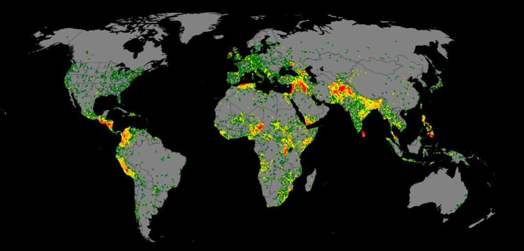
Here Global Terrorism Database (GTD) is used to classify the Terrorist Group which might be involved in an attack based on number of kills, region, weapons used etc.
The tutorial contains a jupyter notebook, which is used to preprocess the data and classify the Terrorist Groups using Machine Learning techniques like Support Vector Machine and Decision Tree with accuracies of 96.55% and 98.27% respectively.
The input and labels of the model are stored in the x_normed.npy and y.npy files respectively.
Further details about the Database can be found in Codebook.pdf file.
import pandas as pd
import numpy as np
import pickle, gzip
import matplotlib.pyplot as plt
from sklearn import svm
from sklearn.metrics import confusion_matrix, precision_recall_fscore_support
from sklearn.tree import DecisionTreeClassifier
from sklearn.preprocessing import MinMaxScaler
from sklearn.model_selection import train_test_split
Removing NA values
df = pd.read_excel('globalterrorismdb_0718dist.xlsx') # reading all data
df.shape
(181691, 135)
df.head()
| iyear | imonth | iday | approxdate | extended | resolution | country | ... | dbsource | INT_LOG | INT_IDEO | INT_MISC | INT_ANY | related | |
|---|---|---|---|---|---|---|---|---|---|---|---|---|---|---|
| 0 | 1970 | 7 | 2 | NaN | 0 | NaT | 58 | ... | PGIS | 0 | 0 | 0 | 0 | NaN |
| 1 | 1970 | 0 | 0 | NaN | 0 | NaT | 130 | ... | PGIS | 0 | 1 | 1 | 1 | NaN |
| 2 | 1970 | 1 | 0 | NaN | 0 | NaT | 160 | ... | PGIS | -9 | -9 | 1 | 1 | NaN |
| 3 | 1970 | 1 | 0 | NaN | 0 | NaT | 78 | ... | PGIS | -9 | -9 | 1 | 1 | NaN |
| 4 | 1970 | 1 | 0 | NaN | 0 | NaT | 101 | ... | PGIS | -9 | -9 | 1 | 1 | NaN |
5 rows × 135 columns
df.isnull().any() # checking columns with null value
eventid               False
iyear                 False
imonth                False
iday                  False
approxdate             True
extended              False
resolution             True
country               False
                      ...
propextent             True
propextent_txt         True
propvalue              True
propcomment            True
ishostkid              True
nhostkid               True
nhostkidus             True
nhours                 True
INT_MISC              False
INT_ANY               False
related                True
Length: 135, dtype: bool
# To remove all columns having null values > 5000
for i in df.columns:
    if df[i].isnull().sum()>5000:
        df.drop(columns=i, inplace=True)
df.shape
(181691, 41)
# further reduction of unnecessary columns after looking at the Codebook (documentation)
df.drop(columns=['eventid', 'extended', 'country_txt', 'region_txt', 'specificity', 'vicinity',
                 'crit1', 'crit2', 'crit3', 'attacktype1_txt', 'targtype1_txt', 'natlty1_txt',
                 'guncertain1', 'individual', 'weaptype1_txt', 'dbsource', 'INT_MISC'], inplace=True)
df.shape
(181691, 24)
# saving file for future use
df.to_csv('terrorist_data_pruned.csv', index=False)
Filling NA values
df2 = pd.read_csv('terrorist_data_pruned.csv')
df2.head()
| iyear | imonth | iday | country | region | provstate | city | ... | natlty1 | gname | weaptype1 | property | ishostkid | INT_LOG | |
|---|---|---|---|---|---|---|---|---|---|---|---|---|---|---|
| 0 | 1970 | 7 | 2 | 58 | 2 | -1 | Santo Domingo | ... | 58.0 | MANO-D | 13 | 0 | 0.0 | 0 |
| 1 | 1970 | 0 | 0 | 130 | 1 | 0 | Mexico city | ... | 21.0 | 23rd of September Communist League | 13 | 0 | 1.0 | 0 |
| 2 | 1970 | 1 | 0 | 160 | 5 | 1 | Unknown | ... | 217.0 | Unknown | 13 | 0 | 0.0 | -9 |
| 3 | 1970 | 1 | 0 | 78 | 8 | 2 | Athens | ... | 217.0 | Unknown | 6 | 1 | 0.0 | -9 |
| 4 | 1970 | 1 | 0 | 101 | 4 | 3 | Fukouka | ... | 217.0 | Unknown | 8 | 1 | 0.0 | -9 |
5 rows × 24 columns
# replacing nan values (refer Codebook.pdf)
df2['doubtterr'].fillna(-9, inplace=True)
df2['multiple'].fillna(0, inplace=True)
df2['natlty1'].fillna(0, inplace=True)
df2['ishostkid'].fillna(-9, inplace=True)
df2['latitude'].fillna(0, inplace=True)
df2['longitude'].fillna(0, inplace=True)

# quantizing dataset
df2['provstate'] = pd.factorize(df2['provstate'])[0]
df2['iyear'] = pd.factorize(df2['iyear'])[0]
df2['city'] = pd.factorize(df2['city'])[0]
df2['country'] = pd.factorize(df2['country'])[0]
df2['target1'] = pd.factorize(df2['target1'])[0]
df2['gname'] = pd.factorize(df2['gname'])[0]
df2['natlty1'] = pd.factorize(df2['natlty1'])[0]

df2.isna().any()
iyear          False
imonth         False
iday           False
country        False
region         False
provstate      False
city           False
latitude       False
longitude      False
doubtterr      False
multiple       False
success        False
suicide        False
attacktype1    False
targtype1      False
target1        False
natlty1        False
gname          False
weaptype1      False
property       False
ishostkid      False
INT_LOG        False
INT_IDEO       False
INT_ANY        False
dtype: bool
# saving file for future use
df2.to_csv('terrorist_data_pruned.csv', index=False)
Normalizing Columns
df = pd.read_csv('terrorist_data_pruned.csv')
df.head()
| iyear | imonth | iday | country | region | provstate | city | latitude | ... | natlty1 | gname | weaptype1 | property | ishostkid | INT_LOG | |
|---|---|---|---|---|---|---|---|---|---|---|---|---|---|---|---|
| 0 | 0 | 7 | 2 | 0 | 2 | 0 | 0 | 18.456792 | ... | 0 | 0 | 13 | 0 | 0.0 | 0 |
| 1 | 0 | 0 | 0 | 1 | 1 | 1 | 1 | 19.371887 | ... | 1 | 1 | 13 | 0 | 1.0 | 0 |
| 2 | 0 | 1 | 0 | 2 | 5 | 2 | 2 | 15.478598 | ... | 2 | 2 | 13 | 0 | 0.0 | -9 |
| 3 | 0 | 1 | 0 | 3 | 8 | 3 | 3 | 37.997490 | ... | 2 | 2 | 6 | 1 | 0.0 | -9 |
| 4 | 0 | 1 | 0 | 4 | 4 | 4 | 4 | 33.580412 | ... | 2 | 2 | 8 | 1 | 0.0 | -9 |
5 rows × 24 columns
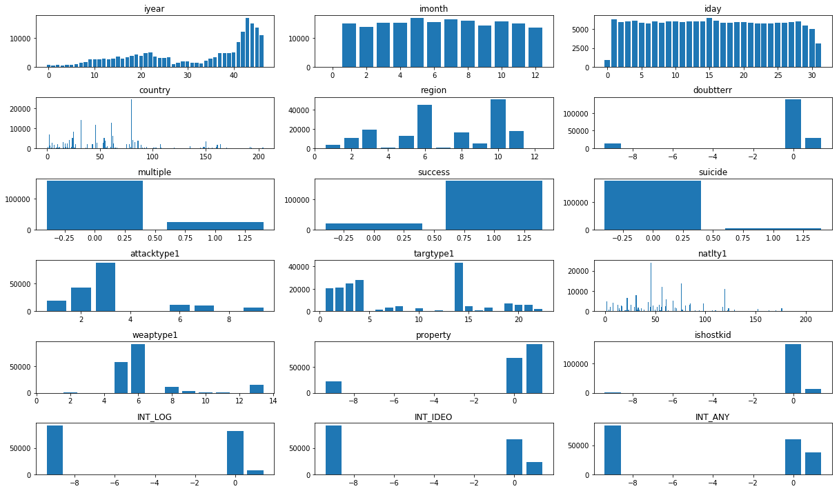
# checking frequency of column values
plt.figure(figsize=(17,10))
i = 0
for col in df.columns:
    if col=='latitude' or col=='longitude' or col=='city' or col=='provstate' or col=='target1' or col=='gname':
        continue
    i += 1
    plt.subplot(6, 3, i)
    num_list = df[col].value_counts()
    plt.bar(num_list.index, num_list.values)
    plt.title(col)
plt.tight_layout()
plt.show()
# classes having less than 600 samples were dropped from the dataframe to remove skewedness in data
num = df['gname'].value_counts()
res = num.where(num>600).dropna()
res
2       82782.0
2001     7478.0
3024     5613.0
455      4555.0
478      3351.0
2699     3288.0
15       2772.0
46       2671.0
203      2487.0
2819     2418.0
1057     2310.0
78       2024.0
2589     1878.0
631      1630.0
221      1606.0
123      1561.0
2695     1351.0
36       1125.0
2632     1062.0
2549     1020.0
948       895.0
1019      830.0
863       716.0
157       639.0
2526      638.0
598       632.0
3136      624.0
281       607.0
Name: gname, dtype: float64
k = []
c = 0
for index, row in df.iterrows():
    if row['gname'] not in list(res.index):
        k.append(index)
    if row['gname']==2:
        c += 1
        if c>5000:
            k.append(index)

df.drop(index=k, inplace=True)
df.shape
(60781, 24)
# converts labels to one-hot encoding
y = pd.get_dummies(df['gname']).values
y.shape
(60781, 28)
# normalizing feature values
x = df.drop(columns='gname')
x = x.values
min_max_scaler = MinMaxScaler()
x_scaled = min_max_scaler.fit_transform(x)
df2 = pd.DataFrame(x_scaled)

x_scaled.shape
(60781, 23)
df2.head()
| 0 | 1 | 2 | 3 | 4 | 5 | 6 | 7 | ... | 17 | 18 | 19 | 20 | 21 | 22 | |
|---|---|---|---|---|---|---|---|---|---|---|---|---|---|---|---|
| 0 | 0.0 | 0.083333 | 0.000000 | 0.010 | 0.363636 | 0.000708 | 0.000082 | 0.572701 | ... | 1.000000 | 0.9 | 0.9 | 0.0 | 0.0 | 1.0 |
| 1 | 0.0 | 0.083333 | 0.000000 | 0.015 | 0.636364 | 0.001062 | 0.000109 | 0.782926 | ... | 0.363636 | 1.0 | 0.9 | 0.0 | 0.0 | 1.0 |
| 2 | 0.0 | 0.083333 | 0.000000 | 0.020 | 0.272727 | 0.001416 | 0.000136 | 0.741690 | ... | 0.545455 | 1.0 | 0.9 | 0.0 | 0.0 | 1.0 |
| 3 | 0.0 | 0.083333 | 0.064516 | 0.025 | 0.000000 | 0.002478 | 0.000218 | 0.781007 | ... | 0.363636 | 1.0 | 0.9 | 0.0 | 0.0 | 0.0 |
| 4 | 0.0 | 0.083333 | 0.258065 | 0.035 | 0.636364 | 0.003540 | 0.000327 | 0.819274 | ... | 0.272727 | 0.9 | 0.9 | 0.0 | 0.0 | 1.0 |
5 rows × 23 columns
# saving file for future use
np.save('x_normed.npy', x_scaled)
np.save('y.npy', y)
Classification
x = np.load('x_normed.npy')
y = np.load('y.npy')

x_train, x_test, y_train, y_test = train_test_split(x, y, test_size=0.1, random_state=0)
print(x_train.shape, y_train.shape, x_test.shape, y_test.shape)
(54702, 23) (54702, 28) (6079, 23) (6079, 28)
model1 = svm.SVC(C=5, kernel='rbf')
model2 = DecisionTreeClassifier()
model1.fit(x_train, np.argmax(y_train, axis=1))
SVC(C=5, cache_size=200, class_weight=None, coef0=0.0,
  decision_function_shape='ovr', degree=3, gamma='auto', kernel='rbf',
  max_iter=-1, probability=False, random_state=None, shrinking=True,
  tol=0.001, verbose=False)
model2.fit(x_train, np.argmax(y_train, axis=1))
DecisionTreeClassifier(class_weight=None, criterion='gini', max_depth=None,
            max_features=None, max_leaf_nodes=None,
            min_impurity_decrease=0.0, min_impurity_split=None,
            min_samples_leaf=1, min_samples_split=2,
            min_weight_fraction_leaf=0.0, presort=False, random_state=None,
            splitter='best')
pred1 = model1.predict(x_test)
acc1 = np.mean(pred1==np.argmax(y_test, axis=1))*100

pred2 = model2.predict(x_test)
acc2 = np.mean(pred2==np.argmax(y_test, axis=1))*100

print('Accuracy SVC: {:.2f}%\nAccuracy Desicion Tree: {:.2f}%'.format(acc1, acc2))
Accuracy SVC: 96.55%
Accuracy Desicion Tree: 98.27%
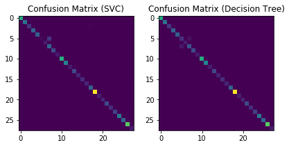
cm1 = confusion_matrix(np.argmax(y_test, axis=1), pred1)
cm2 = confusion_matrix(np.argmax(y_test, axis=1), pred2)

plt.subplot(1, 2, 1)
plt.imshow(cm1)
plt.title('Confusion Matrix (SVC)')

plt.subplot(1, 2, 2)
plt.imshow(cm2)
plt.title('Confusion Matrix (Decision Tree)')

plt.tight_layout()
plt.show()
pr1 = precision_recall_fscore_support(np.argmax(y_test, axis=1), pred1)
pr2 = precision_recall_fscore_support(np.argmax(y_test, axis=1), pred2)

print('SVC\nPrecision: {:.2f}%\nRecall: {:.2f}%\nF-score: {:.2f}%'.format(np.mean(pr1[0])*100, np.mean(pr1[1])*100, np.mean(pr1[2])*100))
print('\nDecision Tree\nPrecision: {:.2f}%\nRecall: {:.2f}%\nF-score: {:.2f}%'.format(np.mean(pr2[0])*100, np.mean(pr2[1])*100, np.mean(pr2[2])*100))
SVC
Precision: 96.12%
Recall: 94.68%
F-score: 94.52%

Decision Tree
Precision: 97.76%
Recall: 97.95%
F-score: 97.84%