Land Classification
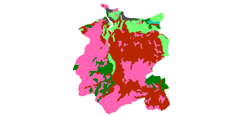
There are multiple satellites that capture the data about the amount of light intensity reflected at different frequencies from the Earth at a very granular geographic level. Some of this information can be used to classify the Earth into different buckets - built-up, barren, green or water. The training data contains different parameters classified into the 4 classes.
Column Description
- Numeric columns X1 to X6 and I1 to I6 define characteristics about the land piece
- ClusterID is a categorical column which clusters a type of land together
- target is the output categorical column which needs to be found for the test dataset
- 1 = Green Land
- 2 = Water
- 3 = Barren Land
- 4 = Built-up
import pandas as pd
import numpy as np
import seaborn as sns
import matplotlib.pyplot as plt
df = pd.read_csv('land_train.csv') # loading the dataset
df.head()
| X1 | X2 | X3 | X4 | X5 | X6 | I1 | I2 | I3 | I4 | I5 | I6 | clusterID | target | |
|---|---|---|---|---|---|---|---|---|---|---|---|---|---|---|
| 0 | 207 | 373 | 267 | 1653 | 886 | 408 | 0.721875 | -1.023962 | 2.750628 | 0.530316 | 0.208889 | 0.302087 | 6 | 1 |
| 1 | 194 | 369 | 241 | 1539 | 827 | 364 | 0.729213 | -1.030143 | 2.668501 | 0.546537 | 0.203306 | 0.300930 | 6 | 1 |
| 2 | 214 | 385 | 264 | 1812 | 850 | 381 | 0.745665 | -1.107047 | 3.000315 | 0.546156 | 0.181395 | 0.361382 | 6 | 1 |
| 3 | 212 | 388 | 293 | 1882 | 912 | 402 | 0.730575 | -1.077747 | 3.006150 | 0.530083 | 0.156835 | 0.347172 | 6 | 1 |
| 4 | 249 | 411 | 332 | 1773 | 1048 | 504 | 0.684561 | -0.941562 | 2.713079 | 0.494370 | 0.205742 | 0.257001 | 6 | 1 |
dfs = df.sample(frac=0.1).reset_index(drop=True) # shuffles the data and takes a fraction of it
dfs.shape
(48800, 14)
Column level preprocessing
Scatter Plot
# scatter plot of a part of data
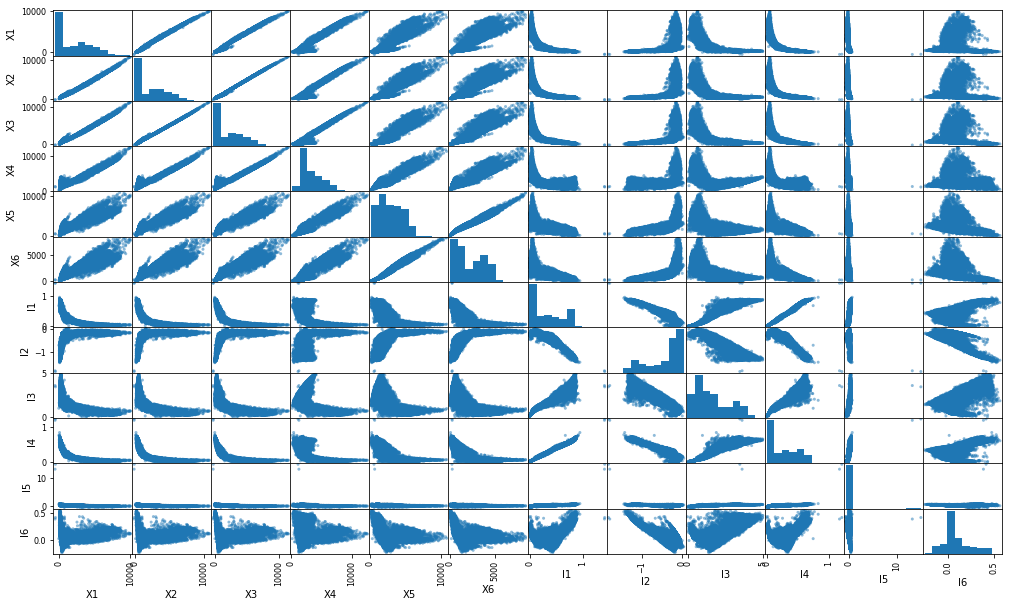
pd.plotting.scatter_matrix(dfs[['X1', 'X2', 'X3', 'X4', 'X5', 'X6', 'I1', 'I2', 'I3', 'I4', 'I5', 'I6']], figsize=(17,10));
Correlation Plot
import seaborn as sns
sns.set(style="white")

# finding correlation
corr = df[['X1', 'X2', 'X3', 'X4', 'X5', 'X6', 'I1', 'I2', 'I3', 'I4', 'I5', 'I6']].corr()

# Generate a mask for the upper triangle
mask = np.zeros_like(corr, dtype=np.bool)
mask[np.triu_indices_from(mask)] = True

# Set up the matplotlib figure
f, ax = plt.subplots(figsize=(11, 9))

# Generate a custom diverging colormap
cmap = sns.diverging_palette(220, 10, as_cmap=True)

# Draw the heatmap with the mask and correct aspect ratio
sns.heatmap(corr, mask=mask, cmap=cmap, vmax=1, center=0.5, square=True, linewidths=.5, cbar_kws={"shrink": .5});
From the scatter plot and correlation plot, we can conclude that-
- The X features are almost linearly correlated with each other. Moreover, they show similar correlation with I features. Therefore, we can merge them into one (average).
- I5 is almost constant and shows less variance (see the histogram). Therefore, it can be dropped.
- I1 and I4 are highly correlated. They can be merged (average).
- I2 shows inverse correlation with I1. It can be dropped.
Remaining columns: Xavg, I14, I3, I6.
Note: Highly correlated columns are dropped since they provide no extra information to the model and hampers the performance.
Selecting features
# preprocessing columns
df['X'] = df[['X1', 'X2', 'X3', 'X4', 'X5', 'X6']].mean(axis=1) # merging all X features in one
df = df.drop(['X1', 'X2', 'X3', 'X4', 'X5', 'X6'], axis=1)      # dropping the rest
df['I14'] = df[['I1', 'I4']].mean(axis=1)                       # averaging I1 and I4
df = df.drop(['I1', 'I4', 'I2', 'I5'], axis=1)                  # dropping the rest
df.head()
| I3 | I6 | clusterID | target | X | I14 | |
|---|---|---|---|---|---|---|
| 0 | 2.750628 | 0.302087 | 6 | 1 | 632.333333 | 0.626095 |
| 1 | 2.668501 | 0.300930 | 6 | 1 | 589.000000 | 0.637875 |
| 2 | 3.000315 | 0.361382 | 6 | 1 | 651.000000 | 0.645910 |
| 3 | 3.006150 | 0.347172 | 6 | 1 | 681.500000 | 0.630329 |
| 4 | 2.713079 | 0.257001 | 6 | 1 | 719.500000 | 0.589465 |
df.to_csv('land_train_pruned.csv', index=False) # saving the data
Row level preprocessing
df.describe()
| I3 | I6 | clusterID | target | X | I14 | |
|---|---|---|---|---|---|---|
| count | 487998.000000 | 487998.000000 | 487998.000000 | 487998.000000 | 487998.000000 | 487998.000000 |
| mean | 1.602914 | 0.098514 | 4.180263 | 1.062301 | 2567.438750 | 0.295633 |
| std | 1.106819 | 0.147183 | 1.645535 | 0.350805 | 1840.983848 | 0.250844 |
| min | -0.177197 | -0.297521 | 1.000000 | 1.000000 | -83.666667 | -0.848529 |
| 25% | 0.694444 | 0.016150 | 3.000000 | 1.000000 | 1015.000000 | 0.067379 |
| 50% | 1.267495 | 0.056333 | 3.000000 | 1.000000 | 1839.000000 | 0.188264 |
| 75% | 2.430122 | 0.161845 | 6.000000 | 1.000000 | 4015.666667 | 0.515738 |
| max | 5.663032 | 0.662566 | 8.000000 | 4.000000 | 10682.333333 | 5.755439 |
df.target.value_counts().plot('bar');
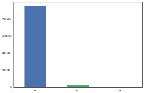
Samples per example:
1: 472987 (97%)
2: 0
3: 14630
4: 381
This clearly shows the imbalance in classes. While training on such data even if the model predits class 1 everytime, the accuracy will be 97%.
Therefore, we need to balance the classes and for this, the approach used is given below.
- Due to very less samples in Class 4, it can be removed.
- Class 1 can be divided randomly into 10 subparts (Samples in each part - 47300).
- Class 3 can be duplicated 2 times (Samples - 43890).
- Trian 10 separate classification models with one part of Class 1 each along with same Class 3 samples in each model.
- Take the average of all models while testing.
Normalizing features
from sklearn import preprocessing

x = df[['I3', 'I6', 'I14', 'X']].values # returns a numpy array
min_max_scaler = preprocessing.MinMaxScaler()
x_scaled = min_max_scaler.fit_transform(x)
df_n = pd.DataFrame(x_scaled, columns=['I3', 'I6', 'I14', 'X'])
df_norm = df[['clusterID', 'target']].join(df_n)

df_norm.head()
| clusterID | target | I3 | I6 | I14 | X | |
|---|---|---|---|---|---|---|
| 0 | 6 | 1 | 0.501320 | 0.624535 | 0.223294 | 0.066506 |
| 1 | 6 | 1 | 0.487258 | 0.623330 | 0.225077 | 0.062481 |
| 2 | 6 | 1 | 0.544073 | 0.686296 | 0.226294 | 0.068240 |
| 3 | 6 | 1 | 0.545072 | 0.671495 | 0.223935 | 0.071073 |
| 4 | 6 | 1 | 0.494891 | 0.577575 | 0.217747 | 0.074602 |
Splitting data into 10 parts
# separating classes
df_1 = df_norm[df_norm.target==1]
df_1 = df_1.sample(frac=1).reset_index(drop=True) # shuffling rows
df_3 = df_norm[df_norm.target==3]

df_1.shape[0], df_3.shape[0]
(472987, 14630)
df_1_split = np.split(df_1, np.arange(47300, 472987, 47300),axis=0) # splits dataframe (of Target=1) in 10
[i.shape for i in df_1_split]
[(47300, 6),
 (47300, 6),
 (47300, 6),
 (47300, 6),
 (47300, 6),
 (47300, 6),
 (47300, 6),
 (47300, 6),
 (47300, 6),
 (47287, 6)]
df_3_dup = pd.concat([df_3]*3, ignore_index=True) # duplicate data (of Target=3) 3 times
df_3_dup.shape
(43890, 6)
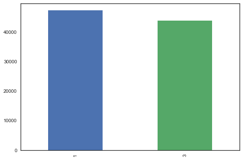
for i in range(len(df_1_split)):
    df_1_split[i] = df_1_split[i].append(df_3_dup, ignore_index=True) # merge Target 1 and 3

[i.shape for i in df_1_split]
[(91190, 6),
 (91190, 6),
 (91190, 6),
 (91190, 6),
 (91190, 6),
 (91190, 6),
 (91190, 6),
 (91190, 6),
 (91190, 6),
 (91177, 6)]
df_1_split[9].target.value_counts().plot('bar');
# saving all parts
for i in range(len(df_1_split)):
    df_1_split[i].to_csv(f'land_train_split_{i+1}.csv', index=False)
Preprocessing Test Data
df_test = pd.read_csv('land_test.csv')
df_test.shape
(2000000, 13)
df_test.head()
| X1 | X2 | X3 | X4 | X5 | X6 | I1 | I2 | I3 | I4 | I5 | I6 | clusterID | |
|---|---|---|---|---|---|---|---|---|---|---|---|---|---|
| 0 | 338 | 554 | 698 | 1605 | 1752 | 1310 | 0.393834 | -0.350045 | 1.565423 | 0.311659 | 0.304781 | -0.043789 | 6 |
| 1 | 667 | 976 | 1187 | 1834 | 1958 | 1653 | 0.214167 | -0.181467 | 1.050679 | 0.196439 | 0.164085 | -0.032700 | 4 |
| 2 | 249 | 420 | 402 | 1635 | 1318 | 736 | 0.605302 | -0.712650 | 2.268984 | 0.441984 | 0.293497 | 0.107348 | 6 |
| 3 | 111 | 348 | 279 | 1842 | 743 | 328 | 0.736917 | -1.162062 | 3.074176 | 0.551699 | 0.080725 | 0.425145 | 6 |
| 4 | 349 | 559 | 642 | 1534 | 1544 | 989 | 0.409926 | -0.406678 | 1.607795 | 0.323984 | 0.212753 | -0.003249 | 6 |
# preprocessing columns
df_test['X'] = df_test[['X1', 'X2', 'X3', 'X4', 'X5', 'X6']].mean(axis=1) # merging all X features in one
df_test = df_test.drop(['X1', 'X2', 'X3', 'X4', 'X5', 'X6'], axis=1)      # dropping the rest
df_test['I14'] = df_test[['I1', 'I4']].mean(axis=1)                       # averaging I1 and I4
df_test = df_test.drop(['I1', 'I4', 'I2', 'I5'], axis=1)                  # dropping the rest
x_test = df_test[['I3', 'I6', 'I14', 'X']].values # returns a numpy array
x_test_scaled = min_max_scaler.transform(x_test)  # applying scaler
df_test_n = pd.DataFrame(x_test_scaled, columns=['I3', 'I6', 'I14', 'X'])
df_test_norm = df_test[['clusterID']].join(df_test_n)
df_test_norm.shape
(2000000, 5)
df_test_norm.head()
| clusterID | I3 | I6 | I14 | X | |
|---|---|---|---|---|---|
| 0 | 6 | 0.298382 | 0.264280 | 0.181902 | 0.104635 |
| 1 | 4 | 0.210245 | 0.275830 | 0.159576 | 0.135875 |
| 2 | 6 | 0.418850 | 0.421701 | 0.207780 | 0.081460 |
| 3 | 6 | 0.556720 | 0.752709 | 0.226051 | 0.064292 |
| 4 | 6 | 0.305637 | 0.306505 | 0.184054 | 0.094727 |
df_test_norm.to_csv('land_test_preprocessed.csv')
Model
from sklearn.tree import DecisionTreeClassifier
from sklearn.neighbors import KNeighborsClassifier
from sklearn.linear_model import LogisticRegression
from sklearn.naive_bayes import GaussianNB
from sklearn.naive_bayes import MultinomialNB
from sklearn.naive_bayes import BernoulliNB
from sklearn.neural_network import MLPClassifier
from sklearn import svm
from sklearn.ensemble import RandomForestClassifier, AdaBoostClassifier
from sklearn.metrics import precision_score, recall_score, f1_score
from sklearn.metrics import confusion_matrix
# different classifiers
num_models = [KNeighborsClassifier(n_neighbors=5), svm.SVC(), LogisticRegression(), GaussianNB(),
              AdaBoostClassifier(), BernoulliNB(), MLPClassifier(),
              RandomForestClassifier(), DecisionTreeClassifier('entropy')]
# training 9 different model on different data splits
# taking average of 9 predictions while testing
# testing set is the 10th data split

models = []
for i in range(9):
    df_train = pd.read_csv('land_train_split_{}.csv'.format(i+1))
    df_train = df_train.sample(frac=1).reset_index(drop=True)

    x = df_train.drop('target', axis=1).values
    y = df_train.target.values

    model = num_models[7]
    models.append(model.fit(x, y))

    print(f'Model {i+1} trained.', end='\r')
Model 9 trained.
# loading the test set
df_test = pd.read_csv('land_train_split_10.csv')
df_test = df_test.sample(frac=1).reset_index(drop=True)

x_test = df_test.drop('target', axis=1).values
y_test = df_test.target.values
# making predictions
predictions = []
for i in range(9):
    predictions.append(list(models[i].predict(x_test)))
predictions = np.array(predictions)
# getting the mojority Class

pred_maj = []
for i in range(predictions.shape[1]):
    (values, counts) = np.unique(predictions[:,i], return_counts=True)
    pred_maj.append(values[np.argmax(counts)])
pred_maj = np.array(pred_maj)
print('Accuracy: {:.2f}%'.format(np.mean(pred_maj==y_test)*100))
precision, recall, f1 = precision_score(y_test, pred_maj), recall_score(y_test, pred_maj), f1_score(y_test, pred_maj)
print('Precision: {:.2f}\nRecall: {:.2f}\nF1 score: {:.2f}'.format(precision, recall, f1))
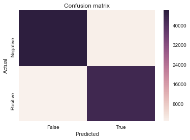
cm = confusion_matrix(y_test, pred_maj, labels=[1,3])
sns.heatmap(cm, xticklabels=['False', 'True'], yticklabels=['Negative', 'Positive'])
plt.xlabel('Predicted')
plt.ylabel('Actual')
plt.title('Confusion matrix');
Accuracy: 97.58%
Precision: 0.98
Recall: 0.97
F1 score: 0.98
Results
| Classifier | Accuracy | F1 Score |
|---|---|---|
| Decision Tree (Entropy) | 99.11% | 0.99 |
| Decision Tree (Gini) | 99.15% | 0.99 |
| Random Forest | 99.23% | 0.99 |
| KNN | 98.53% | 0.99 |
| Logistic Regression | 91.38% | 0.92 |
| Gaussian Naive Bayes | 89.83% | 0.90 |
| Bernoulli Naive Bayes | 51.86% | 0.68 |
| Adaboost Classifier | 95.87% | 0.90 |
| ANN | 89.83% | 0.90 |
| All | 97.58% | 0.98 |
Getting predictions for test set
df_test_set = pd.read_csv("land_test_preprocessed.csv")
df_test_set.drop('Unnamed: 0', inplace=True, axis=1)
df_test_set.head()
| clusterID | I3 | I6 | I14 | X | |
|---|---|---|---|---|---|
| 0 | 6 | 0.298382 | 0.264280 | 0.181902 | 0.104635 |
| 1 | 4 | 0.210245 | 0.275830 | 0.159576 | 0.135875 |
| 2 | 6 | 0.418850 | 0.421701 | 0.207780 | 0.081460 |
| 3 | 6 | 0.556720 | 0.752709 | 0.226051 | 0.064292 |
| 4 | 6 | 0.305637 | 0.306505 | 0.184054 | 0.094727 |
# predictions
predictions = []
for i in range(9):
    predictions.append(list(models[i].predict(df_test_set.values)))
predictions = np.array(predictions)
# getting the mojority Class
pred_maj = []
for i in range(predictions.shape[1]):
    (values, counts) = np.unique(predictions[:,i], return_counts=True)
    pred_maj.append(values[np.argmax(counts)])
pred_maj = np.array(pred_maj)

pred_maj.shape
(2000000,)
df_sub = pd.DataFrame(pred_maj, columns=['target'])
df_sub.head()
| target | |
|---|---|
| 0 | 3 |
| 1 | 3 |
| 2 | 1 |
| 3 | 1 |
| 4 | 3 |
df_sub.to_csv('submission.csv', index=False)
Analysis
dfa = pd.read_csv('land_train_split_1.csv')
dfa.groupby(dfa.target).describe().T
| target | 1 | 3 | |
|---|---|---|---|
| I14 | count | 47300.000000 | 43890.000000 |
| mean | 0.172823 | 0.178143 | |
| std | 0.038544 | 0.010856 | |
| min | 0.126043 | 0.128314 | |
| 25% | 0.138245 | 0.172255 | |
| 50% | 0.153272 | 0.177356 | |
| 75% | 0.208025 | 0.183939 | |
| max | 0.313051 | 0.236896 | |
| I3 | count | 47300.000000 | 43890.000000 |
| mean | 0.303832 | 0.300403 | |
| std | 0.192337 | 0.065502 | |
| min | 0.005789 | 0.024574 | |
| 25% | 0.145690 | 0.265956 | |
| 50% | 0.234960 | 0.289333 | |
| 75% | 0.455870 | 0.326778 | |
| max | 0.908952 | 0.874047 | |
| I6 | count | 47300.000000 | 43890.000000 |
| mean | 0.418548 | 0.235797 | |
| std | 0.151682 | 0.076489 | |
| min | 0.077088 | 0.029555 | |
| 25% | 0.330767 | 0.190215 | |
| 50% | 0.371948 | 0.218487 | |
| 75% | 0.483560 | 0.258432 | |
| max | 0.947382 | 0.818775 | |
| X | count | 47300.000000 | 43890.000000 |
| mean | 0.251571 | 0.131445 | |
| std | 0.172705 | 0.032215 | |
| min | 0.015047 | 0.061382 | |
| 25% | 0.101817 | 0.112948 | |
| 50% | 0.202729 | 0.126339 | |
| 75% | 0.388372 | 0.142888 | |
| max | 0.992523 | 0.519661 | |
| clusterID | count | 47300.000000 | 43890.000000 |
| mean | 4.127294 | 5.833698 | |
| std | 1.634507 | 0.906823 | |
| min | 1.000000 | 1.000000 | |
| 25% | 3.000000 | 6.000000 | |
| 50% | 3.000000 | 6.000000 | |
| 75% | 6.000000 | 6.000000 | |
| max | 8.000000 | 8.000000 |
estimator = models[0].estimators_[5]

from sklearn.tree import export_graphviz
# Export as dot file
export_graphviz(estimator, out_file='tree.dot',
                feature_names = ['clusterID', 'I3', 'I6', 'I14', 'X'],
                class_names = ['1', '3'],
                rounded = True, proportion = False,
                precision = 2, filled = True)

# Convert to png using system command (requires Graphviz)
import pydot
(graph,) = pydot.graph_from_dot_file('tree.dot')
graph.write_png('somefile.png')
# taking sum of all GINI indexes
a = models[0].feature_importances_
for i in range(8):
    a += models[i+1].feature_importances_

a
array([2.10152634, 0.58177282, 3.40019577, 2.06218839, 0.85431669])
The model cannot be visualized because of its size, so I have taken the sum of gini index of attributes, which are shown below.
clusterID: 2.10
I3: 0.58
I6: 3.40
I14: 2.06
X: 0.85
Clearly, I6 classifies the data best.