Ship Detection

Introduction

Object detection is a technology related to computer vision and image processing for detecting various kinds of semantic objects: like cars, trees, person, and so on, from images or video frames. Their application can be found in self-driving cars, video surveillance, object tracking, image retrieval, medical imaging systems, etc. With the traditional image processing methods, researchers had a tough time devising and generalizing the algorithm for various use-cases and that too with reasonable accuracy. While contemporary Deep Learning algorithms have made this task a child’s play. With Object Detection apps on Play store, Nvidia’s Digits framework and a plethora of online tutorials, one can build and use this application with ease.

Satellite images, on the other hand, are becoming an amazing source of contextual information for many industries. They are made of millions of pixels with a variety of ground resolutions ranging from 30cm to 30m. The ground resolution of the images determines the size of the objects that can be detected with them. Images can be multi-spectral, and different spectral bands show different visibility behavior in function of weather events (such as clouds or storms), or simply the time of the day. Application of satellite images can be seen in land cover change detection, monitoring natural calamities like floods and fires, or object detection like buildings, constructions, ponds, and vehicles.

In this tutorial, I would be talking about how to build your object detection algorithm from scratch, which will work on satellite imagery. For this, I would like you to have a little knowledge about Deep Learning, Python, and some terminal commands, that’s all you require. We’ll be using YOLO, a very accurate and fast deep learning algorithm for object detection given by Joseph Redmon et al., hats off to these guys. And with their latest version YOLOv3, the accuracy has been further enhanced. So here we go.

1. Getting Images

There are various government and private organizations providing satellite imageries at different resolutions like Landsat, Sentinel, Planet Labs, and Digital Globe etc. Landsat and Sentinel imageries are easy to acquire through the Google Earth Engine, but they provide a pretty bad resolution, 30m for Landsat and 10m for Sentinel, which is unsuitable for this task. Other possible options are Planet Labs and Digital Globe, but their images are not available for free. Planet Labs, though, have their Education and Research program for students and faculties through which limited access can be acquired on the institutional emails.

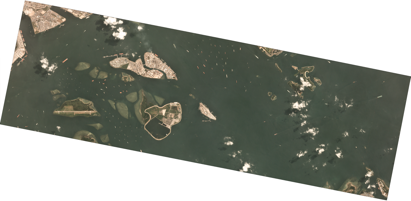
Fig 1. A sample PlanetScope image tile (3m resolution).

If you do not have an institutional email or cannot get the access by any means, a few sample images can be downloaded through this link.

1.1. Planet Labs

Planet Labs is a private Earth-imaging company providing satellite images at different resolutions. The best part is that they monitor the whole Earth daily, which gives access to a massive amount of data. For this task, PlanetScope satellite was used with images at a resolution of 3m, which is enough to detect big ships in the ocean. The images were downloaded through their python API, which requires the API key. Once you sign up for a Planet account, the API key can be retrieved from the profile dashboard.

Fig 2. The geometry of the Area Of Interest (AOI) can be acquired from the geojson.io website.

from planet import api

client = api.ClientV1(api_key='your-api-key')

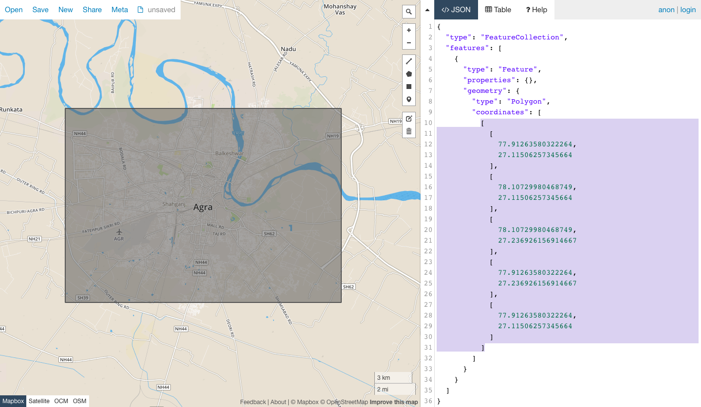
# AOI geometry
bb = [[114.08, 22.31], [114.08, 22.36], [114.16, 22.36], [114.16, 22.31], [114.08, 22.31]]

aoi = {
  "type": "Polygon",
  "coordinates": [bb],
}

max_cloud_percentage = 0.1

# build a filter for the AOI
query = api.filters.and_filter(
  api.filters.geom_filter(aoi),
  api.filters.range_filter('cloud_cover', gt=0),
  api.filters.range_filter('cloud_cover', lt=max_cloud_percentage)
)

# we are requesting PlanetScope 3 Band imagery
item_types = ['PSScene3Band']
request = api.filters.build_search_request(query, item_types)

# this will cause an exception if there are any API related errors
results = client.quick_search(request)

# directory path to save images
save_dir = 'planet_images'
no_of_images = 5

# items_iter returns an iterator over API response pages
for item in results.items_iter(no_of_images):
    # each item is a GeoJSON feature
    print(item['id'])
    assets = client.get_assets(item).get()
    activation = client.activate(assets['visual'])

    callback = api.write_to_file(directory=save_dir)
    body = client.download(assets['visual'], callback=callback)
    body.await()

The code for downloading the Planet image tiles from their python API.

2. Labeling

Since we are not using any public labeled datasets, we have to annotate the images manually. An open-source annotation tool, LabelMe, was used for this purpose.

Note: if you don’t want to label the images, you can download any public dataset like xView, DOTA, or pull the labeled Planet images from my repository.

2.1 LabelMe

Labelme is a python based open-sourced tool to annotate the image data for object detection, segmentation, and various other tasks. It provides the functionality to load an image; draw shapes like line, circle, rectangle or polygon over the areas of interest; and then save the annotation in .json format including the metadata of the image and the annotation information like their shape, geometry, category, etc.

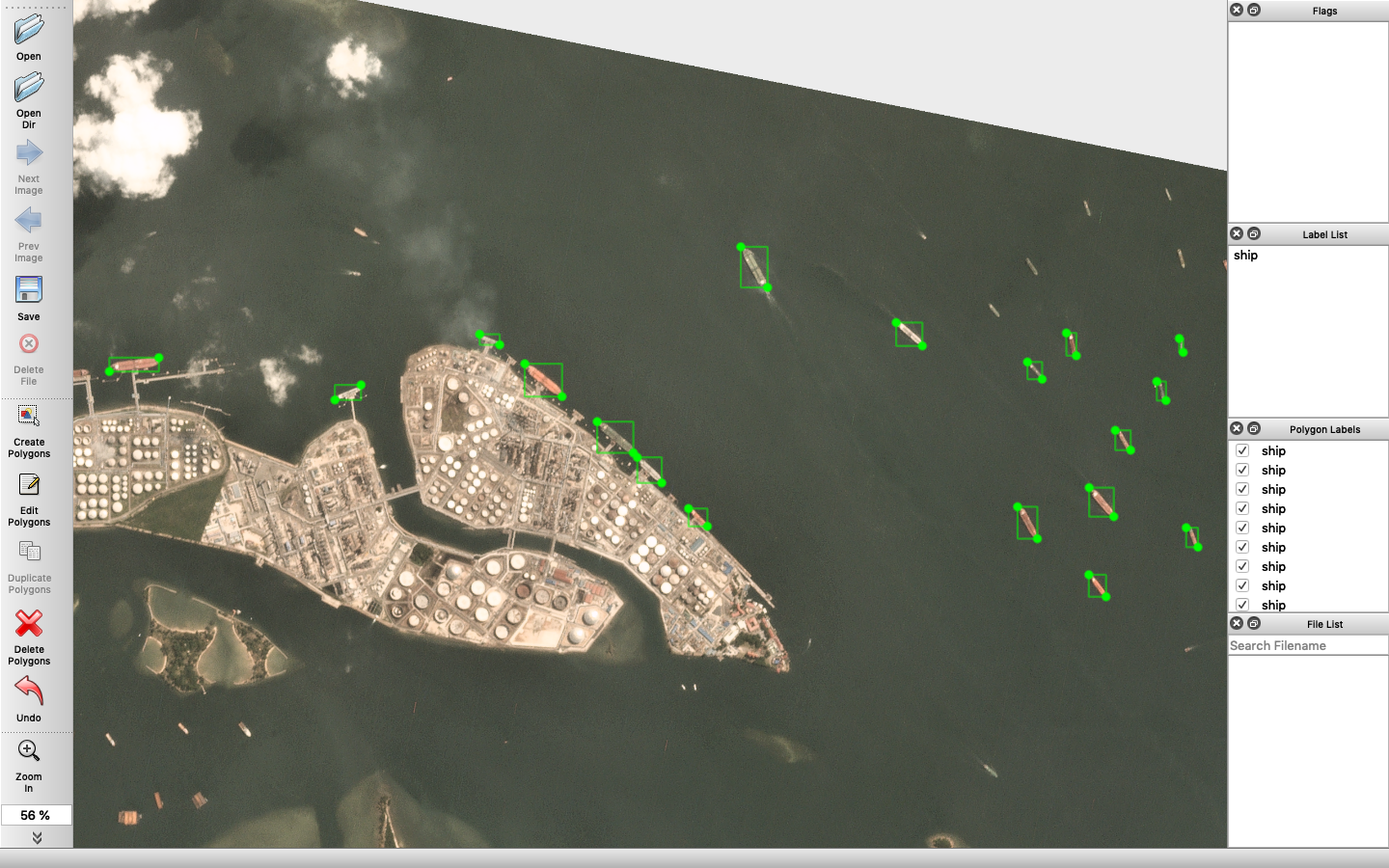
Fig 3. LabelMe annotation tool.

Around 25 Planet image tiles were annotated which were taken from various seaports of the world. There was only one object category, i.e., ship, which made the annotation easier. This could be further extended to ship categories like containers, navy, cargo, passenger, fishing vessels, etc. but requires a little more effort.

2.2 Dividing image in chips

The size of satellite images (around 4500x9000 in this case) makes it very difficult for the network to train, not only due to the variable image dimensions but also because of limited GPU/CPU memory. Therefore, the images were divided into small chips of size 512x512 pixels before feeding to the network. Also, due to the small number of bounding boxes in some images, the centroid of these boxes was clustered using DB-scan algorithm and then divided into chips.

import json
import glob
import numpy as np
from PIL import Image
from scipy.misc import imsave
from sklearn.cluster import DBSCAN

# saves chips of size 512x512
# along with labels in YOLO format
def save_files(image, label, info):
    
    for k in info.keys():
        x, y = info[k]['center'][0], info[k]['center'][1]

        # saving image chip
        iname = 'dataset/{}_{}.png'.format(label['imagePath'][:-4], k)
        imsave(iname, image[y-256:y+256, max(x-256, 0):x+256, :3])

        # saving label
        file = open(iname.replace('.png', '.txt'), 'a')
        for point in info[k]['bbox']:
            [[x_bot, y_bot], [x_top, y_top]] = point
            xc = (x_bot+x_top)//2 - x + 256
            yc = (y_bot+y_top)//2 - y + 256
            w = abs(x_bot-x_top)
            h = abs(y_bot-y_top)

            # 0 means first object i.e. ship
            lab = '0 {} {} {} {}\n'.format(xc/512, yc/512, w/512, h/512)
            file.write(lab)
        file.close()
        
# dividing images into chips
image_folder = 'planet_images'
for file in glob.glob(image_folder+'/*.json'):
    print(file)
    
    # reading files
    with open(file, 'r') as f:
        label = json.load(f)
    image = np.array(Image.open(image_folder+'/'+label['imagePath']))
    
    # extracting coordinates of bounding boxes
    coords, center_list = [], []
    for p in label['shapes']:
        [[x_bot, y_bot], [x_top, y_top]] = p['points']
        coords.append(p['points'])

        # stores box's center coords for clustering
        center_list.append([(x_bot+x_top)//2, (y_bot+y_top)//2])
    coords = np.array(coords)
    
    # DB-Scan algorithm for clustering
    # value of eps (threshold) can be set from 220-256
    # depending on the number of clusters
    eps = 256
    dbscan = DBSCAN(min_samples=1, eps=eps)
    x = np.array(center_list)
    y = dbscan.fit_predict(x)
    
    # storing centroid of clusters
    info = {}
    for i in range(y.max()+1):
        # calculates the max and min coords of all the
        # bounding boxes present in the cluster
        mi_x, mi_y = x[np.where(y==i)[0]].min(axis=0)
        ma_x, ma_y = x[np.where(y==i)[0]].max(axis=0)

        item = {}
        item['center'] = [(mi_x+ma_x)//2, (mi_y+ma_y)//2]
        item['bbox'] = coords[np.where(y==i)[0]].tolist()

        info[i] = item
        
    save_files(image, label, info)

The code for dividing the labeled Planet tiles into chips.

YOLOv3 requires information about the bounding box to be stored in a .txt file. Every object is stored in a separate line where five numbers represent each object. Example: 0 0.45 0.55 0.20 0.11. They are defined in order: object category number, x, and y coordinate of the object center, width, and height of the object. All numbers except the object number, are scaled to [0, 1] by dividing it by the size of the image (512 in our case). Since there was only one category to be detected, the object number in every label file was set to 0.

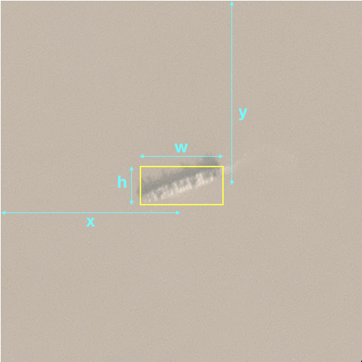
Fig 4. Representation of the object measurements as stored in the label file.

3. YOLO algorithm

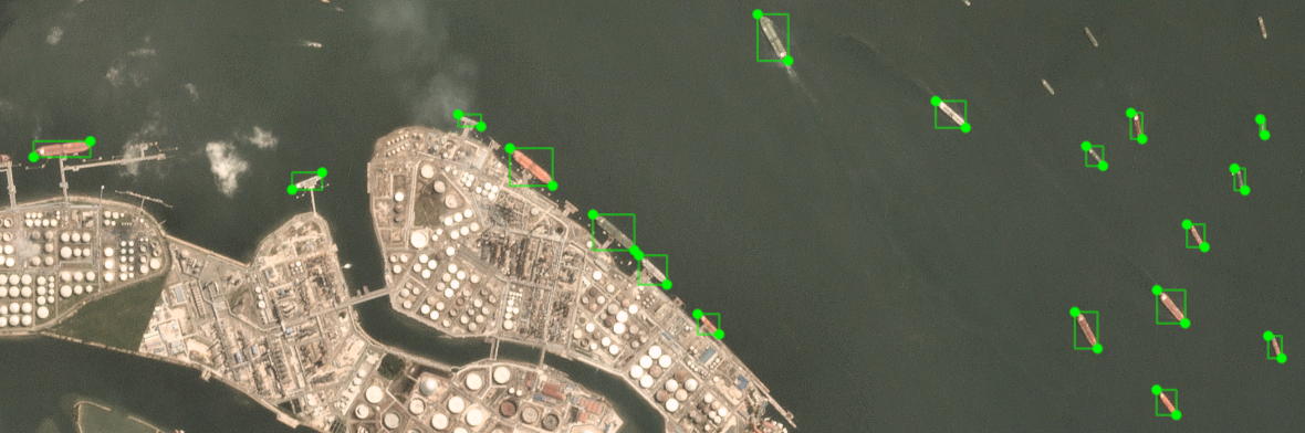
Fig 5. The predictions from the YOLO model.

I’ll be providing a brief introduction to the YOLO algorithm, for a detailed analysis I would suggest you refer this link. Also, here’s a link for the original YOLOv3 paper, which is their latest version.

You Only Look Once is an object detection algorithm touted to be one of the fastest. It was trained on the COCO dataset and achieved a mean Average Precision (mAP) of 33.0 at the speed of 51ms per image on Titan X GPU, which is pretty good. The major highlight of the algorithm is that it divides the input image into several individual grids, and each grid predicts the objects inside it. This way, the whole image is processed at once, and the inference time is reduced.

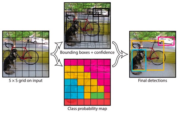
Fig 6. A representation of the YOLO object detection pipeline.

The model is trained on the Darknet Framework, which is an open source neural network framework written in C and CUDA. It is fast, easy to install, and supports CPU and GPU computation. For the ship detection task, we’ll use the same framework. The next sections will guide you through detecting objects with the YOLO system using a pre-trained model.

3.1 Getting Darknet

Getting Darknet is as simple as running these commands in the terminal.

git clone https://github.com/pjreddie/darknet
cd darknet
make

Get the pre-trained weights from here.

wget https://pjreddie.com/media/files/darknet53.conv.74

Try running the detector to confirm the installation.

./darknet detect cfg/yolov3.cfg yolov3.weights data/dog.jpg

You’ll get an output like the one shown in Fig. 7 and a file predictions.jpg will be stored as the output.

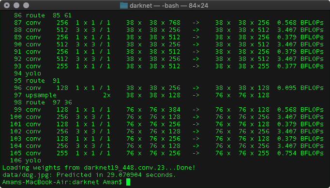
Fig 7. The output after running the detector.

So far, so good. Once the darknet is set up, some files are needed to be added for training on the custom data.

3.2 Preparing the Config files

Darknet requires certain files to know how and what to train. We’ll be creating these files now.

data/ship.names
cfg/ship.data
cfg/yolov3-ship.cfg

.names file contains the name of the object categories you want to detect. If you remember, earlier in the tutorial we provided 0 in the label file which represents the index of the ship. Same order has to be followed while writing in this file. Now, since we have got only one object category, the file will look like the one shown below.

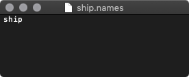
Fig 8. The file containing the name of the object categories to be detected by the algorithm.

This name is shown over the bounding box in the output. For more than one object, every name has to be written in a separate line.

.data file contains information about the training data.

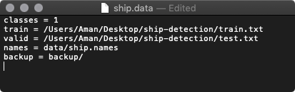
Fig 9. The file containing some information about the input data and backup paths.

The details in this file are pretty much self-explanatory. names variable will contain the path to the object names file you just defined. backup stores the checkpoint of the model during training. The train.txt and test.txt files will contain the path to your training and testing images. And will look something like this:

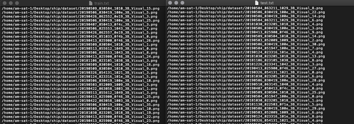
Fig 10. The distribution of training and test images. Both absolute and relative paths will work, but make sure they are valid.

The final step is to set up the .cfg file which contains the information about the YOLO network architecture. For that, just copy the cfg/yolov3.cfg file in the darknet folder, paste it as cfg/yolov3-ship.cfg, and make the following changes:

The variable batch defines the number of images used for one training step, while subdivision is the number of mini-batches. For example, with batch=64 and subdivision=4, one training step will require four mini-batches with 64/4=16 images each before updating the parameters. These variables can be set according to your CPU/GPU memory size.
width and height represent the size of the input image, in our case, it’s 512.
YOLOv3 outputs the boxes in 3 different resolutions, with each label represented by five numbers (i.e., probability/class confidence, x, y, width, and height). Therefore, the number of filters in the last layer is calculated by the formula

filters = (classes + 5) * 3

Since we have got only 1 class, the number of filters become 18. Now replace each occurrence of classes=80 by classes=1 in the file (at line 610, 696, and 783).
Also, replace the filters=255 line by filters=18 each time the classes variable occurs (at line 603, 689, and 776).

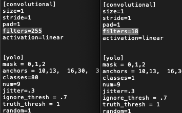
Fig 11. Change the number of classes and filters according to the custom data.

You can even provide the data augmentations while training by adjusting the following variables.
```
angle=0
saturation = 1.5
exposure = 1.5
hue=.1
```

3.3 Training

Before beginning the training process, make sure all the paths provided in the earlier files are correct. The image path in train.txt and test.txt are valid, also their corresponding .txt files are in the same folder. After doing that, run the following command for starting the training procedure.

./darknet detector train cfg/ship.data cfg/yolov3-ship.cfg darknet19_448.conv.23

You’ll get the following output.

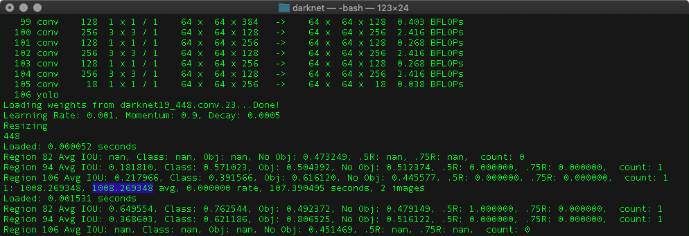
Fig 12. The model logs showing the progression of training.

Here, the highlighted text shows the average loss and should be as low as possible. For the COCO dataset, yolov3 was trained until the average loss reached 0.6. But, this may not be applicable for your dataset; therefore, to make sure that the network doesn’t overfit on the training set, keep on checking its results on the test set.

The backup will be saved in the backup/ folder, use the latest one for testing. Also note that by default the darknet stores the model weights after every 100 iterations till 1000, and after that every 10,000 iterations. Refer line 138 in the examples/detector.c file.

if(i%10000==0 || (i < 1000 && i%100 == 0)){
    ...
  ...
  save_weights(net, buff);
}

You can adjust this according to the speed of your hardware and then recompile darknet using make command. Refer this link for more details.

3.4 Test

Run the following command for testing the trained model.

./darknet detector test cfg/ship.data cfg/yolov3.cfg backup/backup_file.weights test_file.jpg

If you see the model not giving good results or no bounding box at all, wait for the model to train. Sometimes, the average loss may reach somewhere around 2.0-3.0, before the boxes start appearing. This may even be possible due to a small number of training images, so make sure you have collected enough data.

4. Results

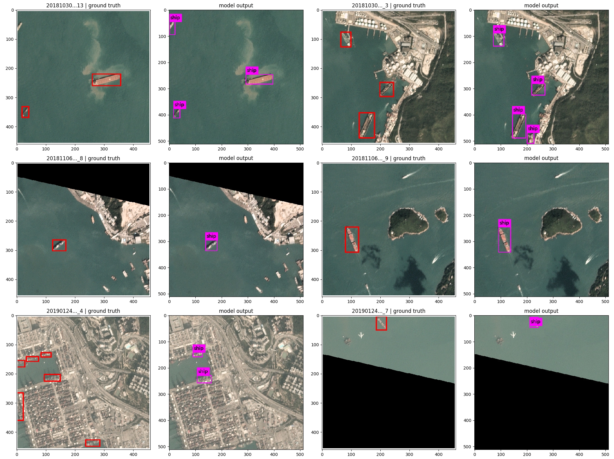
Fig 13. Some results of the model on the test images.

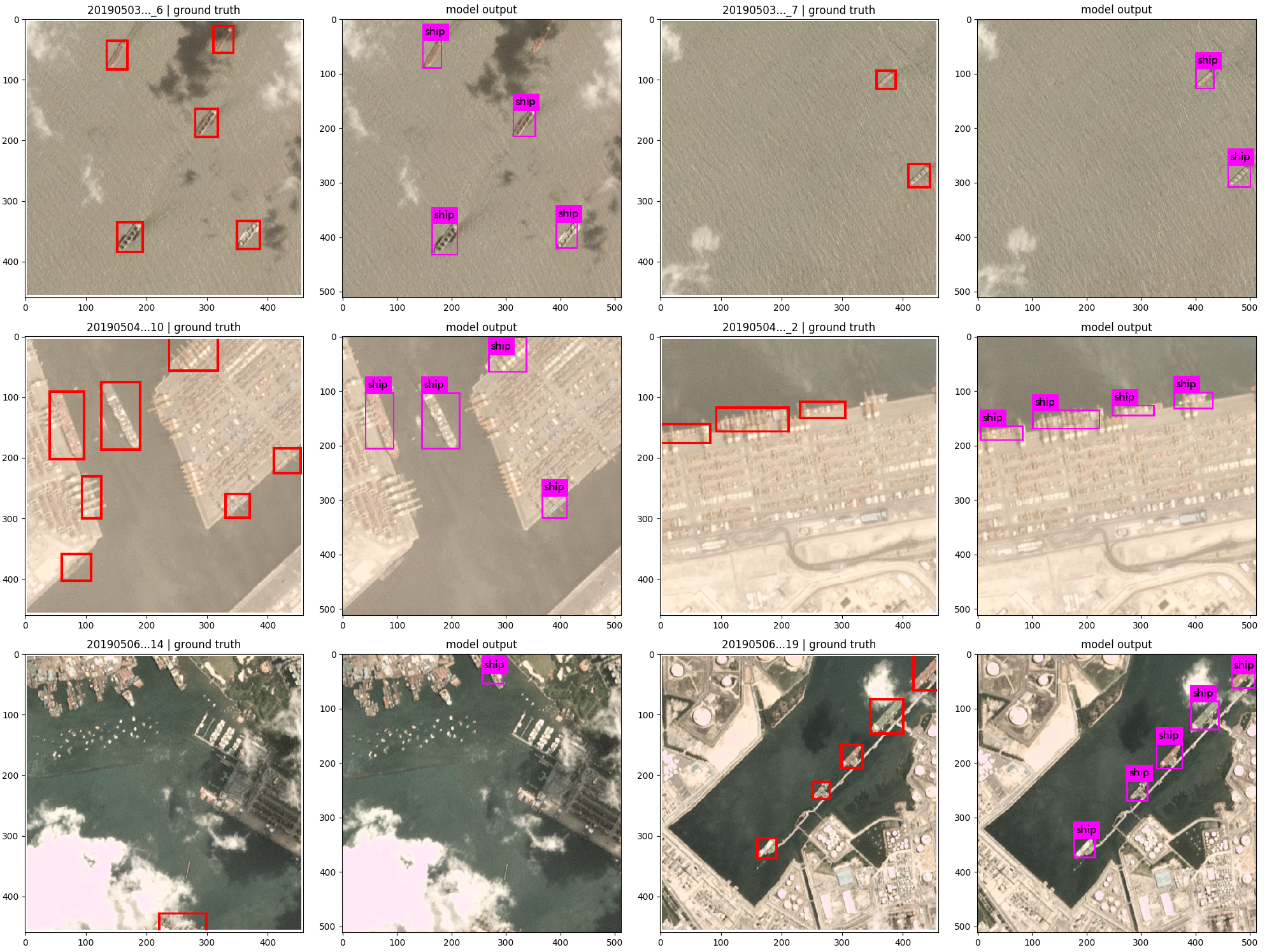
Fig 14. Few more results of the model on the test images.

The model was trained on the AWS EC2 instance using the V100 GPU. With such a powerful accelerator, it took around 1 hr to reach 30,000 iterations with the average loss around 0.9-1.0, and the result was awesome. Except for a few misses here and there, the model worked pretty well on the test set overall. The training set consisted of 200 images, while the test set had 50 images.

In some of the images, the model faced difficulty to detect the ships which were closer to the land, perhaps due to contrast. Ships in the middle of the oceans were easier to detect. Increasing the sample of such images can help the model detect better.

5. Conclusion

Through this tutorial, we learned how to make a custom object detection model to work on satellite images. We first downloaded the RGB imageries form the Planet API, the satellite used in this case was PlanetScope which provides a resolution of 3m. These images were then labeled through an annotation tool, LabelMe, and then converted into chips for convenient usage. The training was done on the YOLOv3 model using the darknet framework, which required a few changes in some files to configure it for the custom data.

The algorithm can be further trained for any object detection dataset by making the required changes in the corresponding files. The full code is available here.

References

https://pjreddie.com/darknet/yolo/
https://timebutt.github.io/static/how-to-train-yolov2-to-detect-custom-objects/
https://www.learnopencv.com/training-yolov3-deep-learning-based-custom-object-detector/
https://towardsdatascience.com/data-science-and-satellite-imagery-985229e1cd2f
Redmon, Joseph and Farhadi, Ali. YOLOv3: An Incremental Improvement. arXiv, 2018.